Scatter Diagram and Correlation Coefficient

 Scatter Diagram and Correlation Coefficient

## Scatter Diagram and Correlation Coefficient

### Scatter Diagram

A **scatter diagram** (or scatter plot) is a graphical representation that displays the relationship between two quantitative variables. Each point on the scatter plot corresponds to an observation in the dataset, with one variable plotted along the X-axis and the other along the Y-axis. This visual representation helps to identify patterns, trends, and potential correlations between the variables.

#### Key Features:

- **Axes**: The horizontal axis (X-axis) typically represents the independent variable, while the vertical axis (Y-axis) represents the dependent variable.

- **Data Points**: Each point on the diagram represents a pair of values from the two variables being analyzed.

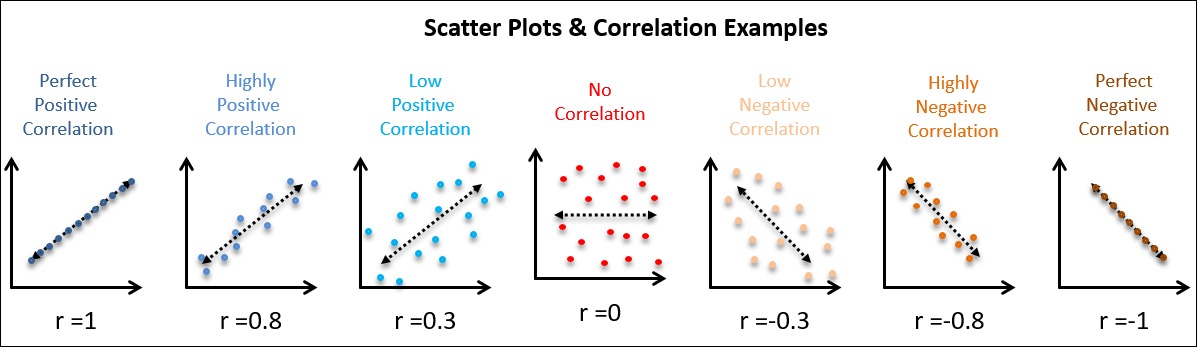
- **Correlation Identification**: The pattern of the plotted points indicates the nature of the relationship:

  - **Positive Correlation**: Points trend upwards from left to right, indicating that as one variable increases, the other also tends to increase.

  - **Negative Correlation**: Points trend downwards from left to right, indicating that as one variable increases, the other tends to decrease.

  - **No Correlation**: Points are scattered without any discernible pattern, suggesting no relationship between the variables.

### Correlation Coefficient

The **correlation coefficient** quantifies the strength and direction of the relationship between two variables. The most commonly used correlation coefficient is **Pearson's correlation coefficient (r)**, which ranges from -1 to +1.

#### Interpretation of Pearson's Correlation Coefficient:

- **+1**: Perfect positive correlation. As one variable increases, the other variable increases perfectly in a linear fashion.

- **0**: No correlation. Changes in one variable do not predict changes in the other variable.

- **-1**: Perfect negative correlation. As one variable increases, the other variable decreases perfectly in a linear fashion.

### Interpretation in a Sociological Study

In a sociological context, interpreting Pearson's correlation coefficient involves understanding the implications of the relationship between two social variables. For example, consider a study examining the relationship between education level (measured in years) and income (measured in dollars).

1. **Positive Correlation (e.g., r = 0.8)**:

   - Interpretation: There is a strong positive correlation between education level and income. This suggests that as education level increases, income tends to increase as well. This finding could support policies aimed at increasing educational access as a means to improve economic outcomes.

2. **No Correlation (e.g., r = 0.0)**:

   - Interpretation: There is no correlation between education level and income. This could indicate that other factors, such as job market conditions or personal circumstances, play a more significant role in determining income than education alone.

3. **Negative Correlation (e.g., r = -0.5)**:

   - Interpretation: A moderate negative correlation might suggest that as one variable increases, the other decreases. For example, if the study found a negative correlation between hours spent on social media and academic performance, it could imply that increased social media use may be associated with lower academic achievement.

### Conclusion

Scatter diagrams and correlation coefficients are essential tools in sociological research for visualizing and quantifying relationships between variables. By interpreting Pearson's correlation coefficient, researchers can draw meaningful conclusions about the nature and strength of associations, informing both theoretical understanding and practical policy implications.

Citations:

[1] https://www.vedantu.com/commerce/scatter-diagram

[2] https://byjus.com/commerce/scatter-diagram/

[3] https://asq.org/quality-resources/scatter-diagram

[4] https://www.geeksforgeeks.org/scatter-diagram-correlation-meaning-interpretation-example/

[5] https://byjus.com/maths/scatter-plot/

[6] https://en.wikipedia.org/wiki/Spearman%27s_rank_correlation_coefficient

[7] https://www.westga.edu/academics/research/vrc/assets/docs/ChiSquareTest_LectureNotes.pdf

[8] https://byjus.com/maths/chi-square-test/

One-Sample Z Test

 One-Sample Z Test

The **one-sample Z test**, **t-test**, and **F test** are statistical methods used to analyze data and test hypotheses in various research situations. Each test has specific applications based on sample size, data distribution, and the nature of the hypothesis being tested. Below is a detailed comparison of these tests, including when to use each.

## One-Sample Z Test

### Definition

The one-sample Z test is used to determine whether the mean of a single sample differs significantly from a known population mean when the population variance is known. It is applicable primarily when the sample size is large (typically $$n \geq 30$$).

### When to Use

- **Large Sample Size**: When the sample size is 30 or more.

- **Known Population Variance**: When the population standard deviation is known.

- **Normal Distribution**: When the data is approximately normally distributed.

### Example

A researcher wants to test if the average height of a sample of students differs from the known average height of students in the population, which is 170 cm. If the sample size is 50 and the population standard deviation is known, a Z test would be appropriate.

## T-Test

### Definition

The t-test is used to compare the means of one or two groups when the population variance is unknown and the sample size is small (typically $$n < 30$$). There are different types of t-tests, including one-sample, independent samples, and paired samples t-tests.

### When to Use

- **Small Sample Size**: When the sample size is less than 30.

- **Unknown Population Variance**: When the population standard deviation is not known.

- **Normal Distribution**: When the data is normally distributed.

### Example

If a researcher wants to determine whether the average test score of a class of 25 students is significantly different from the national average score of 75, they would use a one-sample t-test.

## F Test

### Definition

The F test is used to compare the variances of two or more groups. It is often employed in the context of ANOVA (Analysis of Variance) to determine if there are any statistically significant differences between the means of multiple groups.

### When to Use

- **Comparing Variances**: When the goal is to assess whether the variances of two or more groups are significantly different.

- **Multiple Groups**: When comparing means across multiple groups (more than two).

### Example

A researcher may use an F test to compare the variances of test scores among three different teaching methods to see if one method has more variability than the others.

## Summary of Differences

| Test Type        | Sample Size Requirement | Known Variance | Purpose                                   | Example Application                                     |

|------------------|-------------------------|----------------|-------------------------------------------|--------------------------------------------------------|

| One-Sample Z Test| $$n \geq 30$$           | Known          | Compare sample mean to a known population mean | Testing if average height of students differs from a known average |

| T-Test           | $$n < 30$$              | Unknown        | Compare sample mean to a known population mean or compare means of two groups | Testing if average test scores of a small class differ from national average |

| F Test           | Any size                | Not applicable | Compare variances of two or more groups   | Comparing variances of test scores among different teaching methods |

## Conclusion

Understanding the differences between the one-sample Z test, t-test, and F test is crucial for selecting the appropriate statistical method based on the research design, sample size, and data characteristics. Each test serves a specific purpose, helping researchers draw valid conclusions from their data.

Citations:

[1] https://brandalyzer.blog/2010/12/05/difference-between-z-test-f-test-and-t-test/

[2] https://www.cuemath.com/data/z-test/

[3] https://testbook.com/key-differences/difference-between-t-test-and-f-test

[4] https://www.shiksha.com/online-courses/articles/difference-between-z-test-and-t-test-blogId-158833

[5] https://www.ncbi.nlm.nih.gov/pmc/articles/PMC6813708/

[6] https://www.investopedia.com/terms/z/z-test.asp

[7] https://www.simplilearn.com/tutorials/statistics-tutorial/z-test-vs-t-test

[8] https://www.scribbr.com/statistics/chi-square-tests/

Rationale for Analyzing Ordinal-Scale Data

 Rationale for Analyzing Ordinal-Scale Data

## Rationale for Analyzing Ordinal-Scale Data

Ordinal-scale data is characterized by its ranking order, where the values indicate relative positions but do not specify the magnitude of differences between them. Analyzing ordinal data is important in sociological research for several reasons:

1. **Capturing Order**: Ordinal data allows researchers to capture the order of responses or observations, which is crucial in understanding preferences, attitudes, or levels of agreement. For example, survey responses such as "strongly agree," "agree," "neutral," "disagree," and "strongly disagree" provide valuable insights into public opinion.

2. **Flexibility in Analysis**: Ordinal data can be analyzed using non-parametric statistical methods, making it suitable for situations where the assumptions of parametric tests (like normality) are not met. This flexibility enables researchers to draw meaningful conclusions from a wider range of data types.

3. **Comparative Analysis**: By ranking data, researchers can compare groups or conditions more effectively. For instance, analyzing customer satisfaction ratings across different service providers can highlight which provider is perceived as the best or worst.

4. **Understanding Trends**: Analyzing ordinal data can reveal trends over time or across different groups. For example, tracking changes in public health perceptions before and after a health campaign can inform future interventions.

### Interpreting the Results of a Rank Correlation Coefficient

The rank correlation coefficient, such as Spearman's rank correlation coefficient, is used to assess the strength and direction of the relationship between two ordinal variables. Here’s how to interpret the results:

1. **Coefficient Range**: The rank correlation coefficient (denoted as $$ \rho $$ or $$ r_s $$) ranges from -1 to +1.

   - **+1** indicates a perfect positive monotonic relationship, meaning as one variable increases, the other variable also increases consistently.

   - **-1** indicates a perfect negative monotonic relationship, where an increase in one variable corresponds to a decrease in the other.

   - **0** indicates no correlation, suggesting that changes in one variable do not predict changes in the other.

2. **Strength of the Relationship**: The closer the coefficient is to +1 or -1, the stronger the relationship between the two variables. For example:

   - A coefficient of **0.8** suggests a strong positive correlation, indicating that higher ranks in one variable are associated with higher ranks in the other.

   - A coefficient of **-0.3** suggests a weak negative correlation, indicating a slight tendency for higher ranks in one variable to be associated with lower ranks in the other.

3. **Monotonic Relationships**: It is essential to note that the Spearman rank correlation assesses monotonic relationships, meaning the relationship does not have to be linear. This makes it particularly useful for ordinal data, where the exact differences between ranks are not known.

4. **Causation vs. Correlation**: While a significant rank correlation indicates a relationship between the two variables, it does not imply causation. Researchers must be cautious in interpreting the results and consider other factors that may influence the observed relationship.

5. **Statistical Significance**: The significance of the correlation coefficient can be tested using hypothesis testing. A p-value is calculated to determine whether the observed correlation is statistically significant. A common threshold for significance is $$ p < 0.05 $$, indicating that there is less than a 5% probability that the observed correlation occurred by chance.

### Conclusion

Analyzing ordinal-scale data is vital in sociological research as it captures the ranking of responses and allows for flexible statistical analysis. The rank correlation coefficient, such as Spearman's $$ \rho $$, provides a valuable tool for interpreting relationships between ordinal variables, helping researchers understand trends and associations while being mindful of the distinction between correlation and causation.

Citations:

[1] https://www.technologynetworks.com/tn/articles/spearman-rank-correlation-385744

[2] https://study.com/academy/lesson/spearman-s-rank-correlation-coefficient.html

[3] https://www.simplilearn.com/tutorials/statistics-tutorial/spearmans-rank-correlation

[4] https://en.wikipedia.org/wiki/Spearman%27s_rank_correlation_coefficient

[5] https://journals.lww.com/anesthesia-analgesia/fulltext/2018/05000/correlation_coefficients__appropriate_use_and.50.aspx

[6] https://www.statstutor.ac.uk/resources/uploaded/spearmans.pdf

[7] https://statistics.laerd.com/statistical-guides/spearmans-rank-order-correlation-statistical-guide-2.php

[8] https://datatab.net/tutorial/spearman-correlation

Chi-Square Test

Chi-Square Test

The chi-square test is a fundamental statistical tool used in the bivariate analysis of nominal-scale data. It helps researchers determine whether there is a significant association between two categorical variables. Below is an explanation of how the chi-square test is applied in this context and the role of the level of significance in the analysis.

## Chi-Square Test in Bivariate Analysis of Nominal-Scale Data

### Purpose of the Chi-Square Test

The chi-square test assesses whether the observed frequencies of occurrences in different categories of two nominal variables differ significantly from what would be expected if there were no association between the variables. This is particularly useful in sociological research, where understanding relationships between categorical variables—such as gender, ethnicity, or educational attainment—is crucial.

### How the Chi-Square Test Works

1. **Formulating Hypotheses**:

   - **Null Hypothesis (H0)**: Assumes that there is no significant association between the two variables (i.e., the variables are independent).

   - **Alternative Hypothesis (H1)**: Assumes that there is a significant association between the two variables (i.e., the variables are dependent).

2. **Creating a Contingency Table**: 

   - Data is organized into a contingency table, which displays the frequency counts for each combination of the two categorical variables. Each cell in the table represents the observed frequency for that combination.

3. **Calculating Expected Frequencies**:

   - Expected frequencies are calculated based on the assumption that the null hypothesis is true. This involves determining what the frequencies would be if there were no association between the variables.

4. **Computing the Chi-Square Statistic**:

   - The chi-square statistic is calculated using the formula:

   $$

   \chi^2 = \sum \frac{(O_i - E_i)^2}{E_i}

   $$

   where $$O_i$$ represents the observed frequency, and $$E_i$$ represents the expected frequency for each category.

5. **Determining the Degrees of Freedom**:

   - The degrees of freedom for the test are calculated as:

   $$

   df = (r - 1)(c - 1)

   $$

   where $$r$$ is the number of rows and $$c$$ is the number of columns in the contingency table.

6. **Comparing with Critical Values**:

   - The calculated chi-square statistic is compared to a critical value from the chi-square distribution table based on the degrees of freedom and the chosen level of significance.

### Role of the Level of Significance

The level of significance (often denoted as alpha, typically set at 0.05) is a threshold that determines whether the null hypothesis can be rejected. It represents the probability of making a Type I error, which occurs when the null hypothesis is incorrectly rejected.

- **Interpreting the p-value**: After calculating the chi-square statistic, researchers obtain a p-value that indicates the probability of observing the data if the null hypothesis were true. 

  - If the p-value is less than or equal to the level of significance (e.g., p ≤ 0.05), the null hypothesis is rejected, suggesting that there is a statistically significant association between the two variables.

  

  - Conversely, if the p-value is greater than the level of significance (e.g., p > 0.05), the null hypothesis is not rejected, indicating insufficient evidence to claim an association.

### Example Application

For instance, a sociologist might want to investigate whether there is a relationship between gender (male, female) and preference for a particular political party (Party A, Party B, Party C). By conducting a chi-square test, the researcher can analyze the contingency table of observed frequencies and determine if the distribution of political preferences differs significantly between genders.

### Conclusion

The chi-square test is a powerful method for analyzing bivariate relationships between nominal-scale data in sociological research. By assessing the significance of associations between categorical variables, researchers can gain insights into social behaviors and trends. The level of significance plays a crucial role in this analysis, guiding the decision to accept or reject the null hypothesis and ensuring the validity of the conclusions drawn from the data.

Citations:

[1] https://www.simplilearn.com/tutorials/statistics-tutorial/chi-square-test

[2] https://byjus.com/maths/chi-square-test/

[3] https://www.scribbr.com/statistics/chi-square-tests/

[4] https://www.westga.edu/academics/research/vrc/assets/docs/ChiSquareTest_LectureNotes.pdf

[5] https://www.statisticssolutions.com/free-resources/directory-of-statistical-analyses/chi-square/

[6] https://www.scribbr.com/statistics/chi-square-test-of-independence/

[7] https://www.bmj.com/about-bmj/resources-readers/publications/statistics-square-one/8-chi-squared-tests

[8] https://www.alooba.com/skills/concepts/statistics/measures-of-central-tendency/