Analysis of Interval- and Ratio-scale Data

Analysis of Interval- and Ratio-scale Data


### Unit IV: Analysis of Interval- and Ratio-scale Data


#### A. **Rationale**

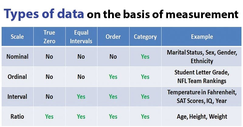
Interval- and ratio-scale data allow for more sophisticated statistical analyses because both scales measure continuous variables. Interval data has meaningful intervals between values, but no true zero point (e.g., temperature in Celsius), while ratio data has a true zero (e.g., income, age). The rationale for analyzing such data is to gain deeper insights into relationships, patterns, and trends, making it possible to perform tests of significance and assess the strength and nature of relationships between variables. This allows researchers to make more precise and reliable inferences about populations.


---


#### B. **Univariate Data Analysis: One-Sample Z, t, and F Tests**


- **Z Test**: A statistical test used to determine whether the mean of a population is significantly different from a hypothesized value when the population variance is known and the sample size is large (n > 30).

  - Formula: 

    \[

    Z = \frac{\bar{X} - \mu}{\sigma / \sqrt{n}}

    \]

    Where:

    - \(\bar{X}\) = Sample mean

    - \(\mu\) = Population mean

    - \(\sigma\) = Population standard deviation

    - \(n\) = Sample size


- **t-Test**: Used when the population variance is unknown and the sample size is small (n < 30). It tests whether the sample mean is significantly different from a hypothesized population mean.

  - Formula:

    \[

    t = \frac{\bar{X} - \mu}{s / \sqrt{n}}

    \]

    Where:

    - \(s\) = Sample standard deviation (used instead of population standard deviation).


- **F Test**: Used to compare the variances of two populations or assess whether multiple group means differ significantly (ANOVA). This test is critical for understanding whether variability between groups is due to chance or a real difference.


---


#### C. **Bivariate Data Analysis**


- **Two-Way Frequency Table**: Similar to nominal data analysis, but in interval/ratio data, the emphasis is more on measuring the strength of the relationship between variables.


- **Scatter Diagram**: A graphical representation that plots two variables on a Cartesian plane. It helps in visualizing the relationship between two interval or ratio variables. The pattern in the scatter diagram provides clues about the direction and strength of the relationship.


- **Correlation Coefficient**: Measures the strength and direction of the relationship between two variables. The most common is **Pearson’s r**, which ranges from -1 to 1. A value close to 1 or -1 indicates a strong relationship, while a value near 0 indicates a weak or no relationship.

  - Formula for Pearson's r:

    \[

    r = \frac{n(\sum xy) - (\sum x)(\sum y)}{\sqrt{[n\sum x^2 - (\sum x)^2][n\sum y^2 - (\sum y)^2]}}

    \]


- **Simple Linear Regression**: A method for predicting the value of a dependent variable based on the value of an independent variable. It establishes a linear relationship between two variables.

  - Formula: 

    \[

    Y = a + bX

    \]

    Where:

    - \(Y\) = Dependent variable

    - \(X\) = Independent variable

    - \(a\) = Intercept

    - \(b\) = Slope (rate of change).


- **Two-Sample Z, t, and F Tests**: These are extensions of the one-sample tests, used when comparing two independent groups:

  - **Two-sample Z Test**: Compares the means of two independent samples when the population variances are known.

  - **Two-sample t-Test**: Used when population variances are unknown, and it tests whether two sample means differ significantly.

  - **Two-sample F Test**: Compares the variances of two independent samples.


- **Significance Tests of Correlation and Regression Coefficients**: These tests determine whether the observed correlation or regression coefficients are statistically significant. The hypothesis test checks if the correlation or slope coefficient is significantly different from zero, indicating a meaningful relationship between the variables.


---


#### D. **Interpretation**

The interpretation of these analyses involves understanding the meaning of the statistical output and its implications. For example:

- In correlation analysis, you interpret the direction (positive or negative) and strength of the relationship.

- In regression analysis, the slope coefficient (\(b\)) indicates the rate of change in the dependent variable for each unit change in the independent variable.

- In significance tests, p-values are used to determine whether the results are statistically significant. A p-value less than 0.05 typically indicates that the relationship or difference is not due to random chance.


---


#### E. **Inference**

Inferences from interval and ratio data analysis help researchers generalize their findings from a sample to the larger population. These tests allow you to make informed conclusions, such as predicting outcomes (e.g., predicting income based on education level), or understanding the strength and nature of relationships between variables in the population. Confidence intervals and hypothesis testing are essential for making these inferences reliable.


---


### **Readings** for this Unit:

1. **Blalock, H.M.** (1969). *Interval Scales: Frequency distribution and graphic presentation* (Chapter 4, pp. 41-54): This chapter covers the basics of summarizing interval-scale data using frequency distributions and visual methods like graphs.

2. **Blalock, H.M.** (1969). *Interval Scales: Measures of Central Tendency* (Chapter 5, pp. 55-76): This reading focuses on the measures of central tendency (mean, median, mode) for interval data.

3. **Blalock, H.M.** (1969). *Two Samples Test: Difference of Means and Proportions* (Chapter 13, pp. 219-242): This chapter explains how to test for significant differences between two samples.

4. **Levin and Fox**, *Elementary Statistics in Social Research*, Chapter 7: "Testing Differences between Means" (pp. 235-268): This reading explains various methods for testing mean differences between groups using z, t, and F tests.

5. **Blalock, H.M.** (1969). *Correlation and Regression* (Chapter 17, pp. 361-396): This chapter provides an in-depth understanding of correlation and regression analysis, crucial for analyzing interval and ratio data.

6. **Levin and Fox**, *Elementary Statistics in Social Research*, Chapters 10 and 11 (pp. 345-392): These chapters further elaborate on correlation and regression analysis, including testing for significance of relationships and interpreting regression coefficients.


These readings will guide you through the theoretical and practical aspects of analyzing interval and ratio-scale data in sociological research. Let me know if you'd like to explore any topic in more detail!


Analysis of Nominal-Scale Data

Analysis of Nominal-Scale Data


### Unit II: Analysis of Nominal-Scale Data


#### A. **Rationale**

Nominal-scale data refers to data that is categorized without any quantitative value or inherent ranking between the categories. These variables represent distinct groups or types, such as gender, ethnicity, religion, or political affiliation. The key rationale for analyzing nominal data is to summarize and compare proportions or frequencies within different categories, as well as to assess relationships between these categories. Since nominal data does not involve a hierarchy or order, only frequency-based analyses are suitable for such data.


Nominal data is often visualized using bar charts or pie charts to show proportions, and it is analyzed using techniques such as frequency tables and contingency tables to explore relationships between variables.


---


#### B. **Univariate Data Analysis: One-Way Frequency Table**

A **one-way frequency table** is used in univariate analysis (the analysis of a single variable) to display the number of occurrences for each category within a nominal variable. This helps in summarizing how often each category appears in a dataset.


For example, if you are analyzing a dataset on political affiliation with categories such as Democrat, Republican, and Independent, a one-way frequency table would display the count of respondents in each category:

| Political Affiliation | Frequency |

|-----------------------|-----------|

| Democrat              | 100       |

| Republican            | 120       |

| Independent           | 80        |


This table provides a clear, simple representation of how the data is distributed across categories.


---


#### C. **Bivariate Data Analysis: Two-Way Frequency Table and Chi-Square Test**


**Two-Way Frequency Table (Contingency Table)**:

A two-way frequency table, also known as a **contingency table**, is used to explore the relationship between two nominal variables. It shows how frequently each combination of categories occurs. For example, a contingency table might compare **political affiliation** with **gender**:


|                | Democrat | Republican | Independent | Total |

|----------------|----------|------------|-------------|-------|

| Male           | 50       | 70         | 30          | 150   |

| Female         | 50       | 50         | 50          | 150   |

| Total          | 100      | 120        | 80          | 300   |


This table can help sociologists assess whether there is an association between gender and political affiliation.


**Chi-Square Test**:

The chi-square test is a statistical test used to determine whether there is a significant association between two nominal variables. It compares the observed frequencies in the contingency table to the expected frequencies (what would occur if there were no association between the variables).


The formula for the chi-square statistic (χ²) is:

\[

\chi^2 = \sum \frac{(O - E)^2}{E}

\]

Where:

- **O** = Observed frequency

- **E** = Expected frequency (calculated under the assumption of no relationship between the variables)


If the calculated chi-square value exceeds a certain threshold (based on the degrees of freedom and significance level), the null hypothesis (no relationship between the variables) is rejected, indicating that a significant association exists.


---


#### D. **Level of Significance (Measures of Strength of Relationship)**

In hypothesis testing, the **level of significance** (denoted by **α**) is the threshold for determining whether to reject the null hypothesis. Typically, α is set at 0.05, meaning that there is a 5% risk of rejecting the null hypothesis when it is actually true (a Type I error).


- **P-value**: The p-value indicates the probability of observing the test results under the assumption that the null hypothesis is true. If the p-value is less than the level of significance (e.g., p < 0.05), the null hypothesis is rejected.

- **Cramér's V**: This is a measure of the strength of association between two nominal variables. Cramér's V ranges from 0 (no association) to 1 (perfect association). It is derived from the chi-square statistic and accounts for the size of the table.


---


#### E. **Interpretation**

The interpretation of results from chi-square tests or frequency tables involves determining whether there is a statistically significant relationship between variables. If the chi-square test shows significance (p < 0.05), it indicates that the observed relationship between the variables is unlikely to have occurred by chance.


- In the context of a two-way table, the interpretation involves looking at whether the distribution across categories deviates from what would be expected under the assumption of no association.

- In addition, the strength of the relationship (using Cramér's V) can help in determining whether the relationship, even if significant, is weak or strong.


For example, in the political affiliation and gender analysis, if the chi-square test is significant, it may suggest that gender is related to political affiliation in the sample.


---


#### F. **Inference**

Inference in nominal-scale data analysis refers to making generalizations about a population based on the analysis of a sample. After conducting tests like chi-square, sociologists can infer whether the relationships observed in the sample likely hold true for the larger population. This is done while acknowledging the limitations of the data, including sample size, potential biases, and random error.


For example, if the chi-square test reveals a significant relationship between gender and political affiliation in the sample, a researcher might infer that gender plays a role in political affiliation in the broader population, assuming the sample is representative.


---


### **Readings** for this Unit:

1. **Blalock, H.M.** (1969). *Nominal Scales: Proportions, Percentages, and Ratios* (Chapter 3, pp. 31-40): This reading focuses on the application of proportions, percentages, and ratios in the analysis of nominal data, providing a detailed understanding of how these tools can summarize nominal-scale data effectively.

2. **Blalock, H.M.** (1969). *Nominal Scales: Contingency Problems* (Chapter 15, pp. 275-316): This chapter delves into the challenges of analyzing relationships between nominal variables using contingency tables and offers solutions for accurately interpreting contingency problems in sociological research.


These readings will deepen your understanding of nominal-scale data analysis and its application in sociological research. Let me know if you'd like further elaboration on any of these topics!


Popular Posts