Rationale for Analyzing Ordinal-Scale Data

 Rationale for Analyzing Ordinal-Scale Data

## Rationale for Analyzing Ordinal-Scale Data

Ordinal-scale data is characterized by its ranking order, where the values indicate relative positions but do not specify the magnitude of differences between them. Analyzing ordinal data is important in sociological research for several reasons:

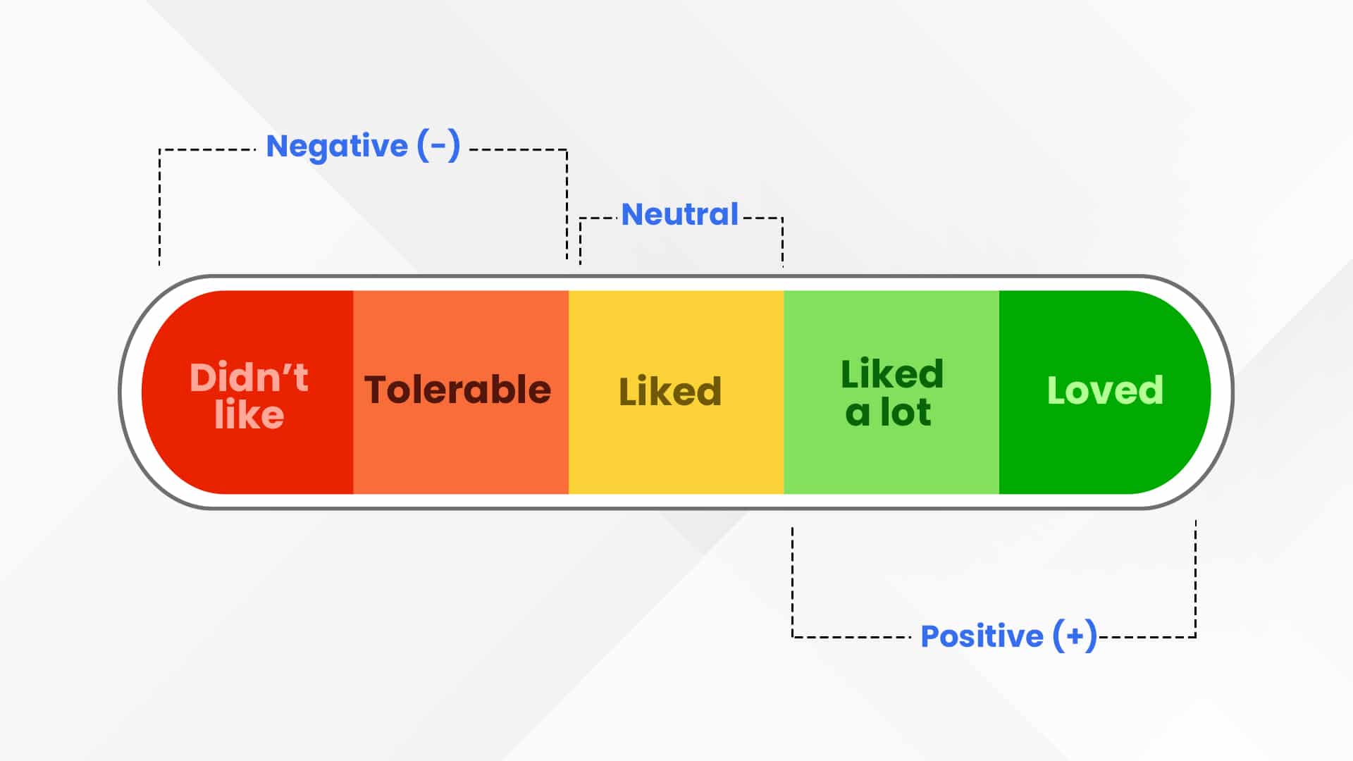
1. **Capturing Order**: Ordinal data allows researchers to capture the order of responses or observations, which is crucial in understanding preferences, attitudes, or levels of agreement. For example, survey responses such as "strongly agree," "agree," "neutral," "disagree," and "strongly disagree" provide valuable insights into public opinion.

2. **Flexibility in Analysis**: Ordinal data can be analyzed using non-parametric statistical methods, making it suitable for situations where the assumptions of parametric tests (like normality) are not met. This flexibility enables researchers to draw meaningful conclusions from a wider range of data types.

3. **Comparative Analysis**: By ranking data, researchers can compare groups or conditions more effectively. For instance, analyzing customer satisfaction ratings across different service providers can highlight which provider is perceived as the best or worst.

4. **Understanding Trends**: Analyzing ordinal data can reveal trends over time or across different groups. For example, tracking changes in public health perceptions before and after a health campaign can inform future interventions.

### Interpreting the Results of a Rank Correlation Coefficient

The rank correlation coefficient, such as Spearman's rank correlation coefficient, is used to assess the strength and direction of the relationship between two ordinal variables. Here’s how to interpret the results:

1. **Coefficient Range**: The rank correlation coefficient (denoted as $$ \rho $$ or $$ r_s $$) ranges from -1 to +1.

   - **+1** indicates a perfect positive monotonic relationship, meaning as one variable increases, the other variable also increases consistently.

   - **-1** indicates a perfect negative monotonic relationship, where an increase in one variable corresponds to a decrease in the other.

   - **0** indicates no correlation, suggesting that changes in one variable do not predict changes in the other.

2. **Strength of the Relationship**: The closer the coefficient is to +1 or -1, the stronger the relationship between the two variables. For example:

   - A coefficient of **0.8** suggests a strong positive correlation, indicating that higher ranks in one variable are associated with higher ranks in the other.

   - A coefficient of **-0.3** suggests a weak negative correlation, indicating a slight tendency for higher ranks in one variable to be associated with lower ranks in the other.

3. **Monotonic Relationships**: It is essential to note that the Spearman rank correlation assesses monotonic relationships, meaning the relationship does not have to be linear. This makes it particularly useful for ordinal data, where the exact differences between ranks are not known.

4. **Causation vs. Correlation**: While a significant rank correlation indicates a relationship between the two variables, it does not imply causation. Researchers must be cautious in interpreting the results and consider other factors that may influence the observed relationship.

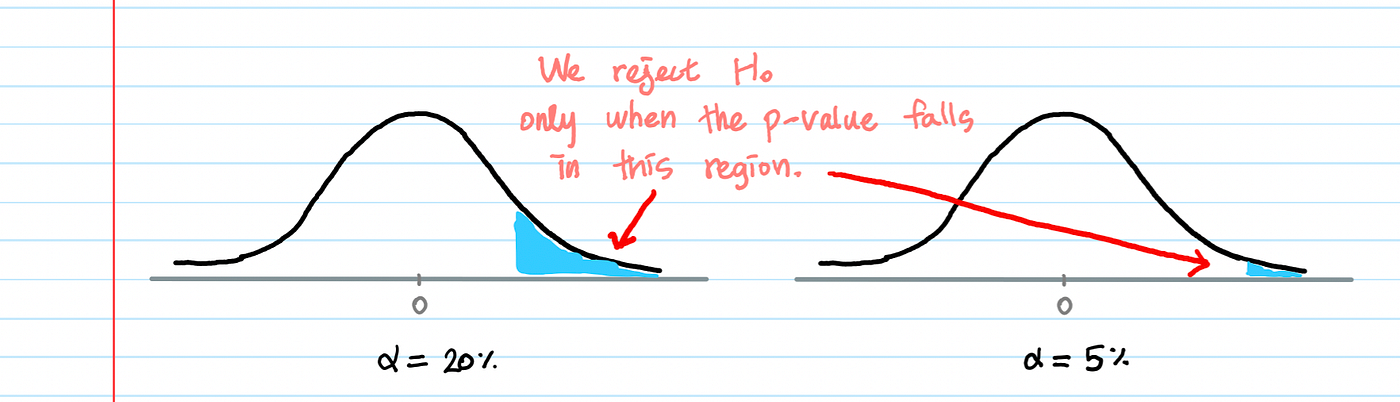
5. **Statistical Significance**: The significance of the correlation coefficient can be tested using hypothesis testing. A p-value is calculated to determine whether the observed correlation is statistically significant. A common threshold for significance is $$ p < 0.05 $$, indicating that there is less than a 5% probability that the observed correlation occurred by chance.

### Conclusion

Analyzing ordinal-scale data is vital in sociological research as it captures the ranking of responses and allows for flexible statistical analysis. The rank correlation coefficient, such as Spearman's $$ \rho $$, provides a valuable tool for interpreting relationships between ordinal variables, helping researchers understand trends and associations while being mindful of the distinction between correlation and causation.

Citations:

[1] https://www.technologynetworks.com/tn/articles/spearman-rank-correlation-385744

[2] https://study.com/academy/lesson/spearman-s-rank-correlation-coefficient.html

[3] https://www.simplilearn.com/tutorials/statistics-tutorial/spearmans-rank-correlation

[4] https://en.wikipedia.org/wiki/Spearman%27s_rank_correlation_coefficient

[5] https://journals.lww.com/anesthesia-analgesia/fulltext/2018/05000/correlation_coefficients__appropriate_use_and.50.aspx

[6] https://www.statstutor.ac.uk/resources/uploaded/spearmans.pdf

[7] https://statistics.laerd.com/statistical-guides/spearmans-rank-order-correlation-statistical-guide-2.php

[8] https://datatab.net/tutorial/spearman-correlation

Chi-Square Test

Chi-Square Test

The chi-square test is a fundamental statistical tool used in the bivariate analysis of nominal-scale data. It helps researchers determine whether there is a significant association between two categorical variables. Below is an explanation of how the chi-square test is applied in this context and the role of the level of significance in the analysis.

## Chi-Square Test in Bivariate Analysis of Nominal-Scale Data

### Purpose of the Chi-Square Test

The chi-square test assesses whether the observed frequencies of occurrences in different categories of two nominal variables differ significantly from what would be expected if there were no association between the variables. This is particularly useful in sociological research, where understanding relationships between categorical variables—such as gender, ethnicity, or educational attainment—is crucial.

### How the Chi-Square Test Works

1. **Formulating Hypotheses**:

   - **Null Hypothesis (H0)**: Assumes that there is no significant association between the two variables (i.e., the variables are independent).

   - **Alternative Hypothesis (H1)**: Assumes that there is a significant association between the two variables (i.e., the variables are dependent).

2. **Creating a Contingency Table**: 

   - Data is organized into a contingency table, which displays the frequency counts for each combination of the two categorical variables. Each cell in the table represents the observed frequency for that combination.

3. **Calculating Expected Frequencies**:

   - Expected frequencies are calculated based on the assumption that the null hypothesis is true. This involves determining what the frequencies would be if there were no association between the variables.

4. **Computing the Chi-Square Statistic**:

   - The chi-square statistic is calculated using the formula:

   $$

   \chi^2 = \sum \frac{(O_i - E_i)^2}{E_i}

   $$

   where $$O_i$$ represents the observed frequency, and $$E_i$$ represents the expected frequency for each category.

5. **Determining the Degrees of Freedom**:

   - The degrees of freedom for the test are calculated as:

   $$

   df = (r - 1)(c - 1)

   $$

   where $$r$$ is the number of rows and $$c$$ is the number of columns in the contingency table.

6. **Comparing with Critical Values**:

   - The calculated chi-square statistic is compared to a critical value from the chi-square distribution table based on the degrees of freedom and the chosen level of significance.

### Role of the Level of Significance

The level of significance (often denoted as alpha, typically set at 0.05) is a threshold that determines whether the null hypothesis can be rejected. It represents the probability of making a Type I error, which occurs when the null hypothesis is incorrectly rejected.

- **Interpreting the p-value**: After calculating the chi-square statistic, researchers obtain a p-value that indicates the probability of observing the data if the null hypothesis were true. 

  - If the p-value is less than or equal to the level of significance (e.g., p ≤ 0.05), the null hypothesis is rejected, suggesting that there is a statistically significant association between the two variables.

  

  - Conversely, if the p-value is greater than the level of significance (e.g., p > 0.05), the null hypothesis is not rejected, indicating insufficient evidence to claim an association.

### Example Application

For instance, a sociologist might want to investigate whether there is a relationship between gender (male, female) and preference for a particular political party (Party A, Party B, Party C). By conducting a chi-square test, the researcher can analyze the contingency table of observed frequencies and determine if the distribution of political preferences differs significantly between genders.

### Conclusion

The chi-square test is a powerful method for analyzing bivariate relationships between nominal-scale data in sociological research. By assessing the significance of associations between categorical variables, researchers can gain insights into social behaviors and trends. The level of significance plays a crucial role in this analysis, guiding the decision to accept or reject the null hypothesis and ensuring the validity of the conclusions drawn from the data.

Citations:

[1] https://www.simplilearn.com/tutorials/statistics-tutorial/chi-square-test

[2] https://byjus.com/maths/chi-square-test/

[3] https://www.scribbr.com/statistics/chi-square-tests/

[4] https://www.westga.edu/academics/research/vrc/assets/docs/ChiSquareTest_LectureNotes.pdf

[5] https://www.statisticssolutions.com/free-resources/directory-of-statistical-analyses/chi-square/

[6] https://www.scribbr.com/statistics/chi-square-test-of-independence/

[7] https://www.bmj.com/about-bmj/resources-readers/publications/statistics-square-one/8-chi-squared-tests

[8] https://www.alooba.com/skills/concepts/statistics/measures-of-central-tendency/